
When using a spreadsheet in Microsoft Excel (Excel) it may help to format the cells containing information to get the best results. The method of doing this will vary in other spreadsheet programs/apps but similar features are likely to exist.
When data is entered into a cell (the intersection of a column and row) of a spreadsheet, the program being used will try and do its best on how to display this information entered. For example if you enter 15.78 then it will, by default, display this as 15.78. However you may not think of the information you entered as a number with two decimal places but as currency, for example, it represents £15.78 or $15.78…
Quite quickly we may see the weakness of allowing the spreadsheet program to try and do its best. Another example may be that you are entering several numbers to three decimal places (e.g. 15.799, 16.101, 101.222, 999.999). These will all display by default to three decimal places. However you may wish to enter 15.799, 20.1, 39, 15.01 and have them all display to three decimal places but by default they will display as shown.
Excel and other spreadsheet programs allow the user to decide the formatting for specific cells or group of cells (such as all cells in a column, all cells in a row or all cells within an area such as columns 3 to 5 within rows 2 to 12). Possibly the easiest way to set formatting it to select a cell or cells (column, row, group) and then a right-mouse click to see open the context sensitive menu (from Excel 2019) as shown below:
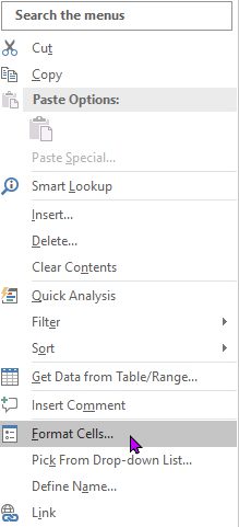
Select Format Cells… and the format cells dialogue window will open showing various options:
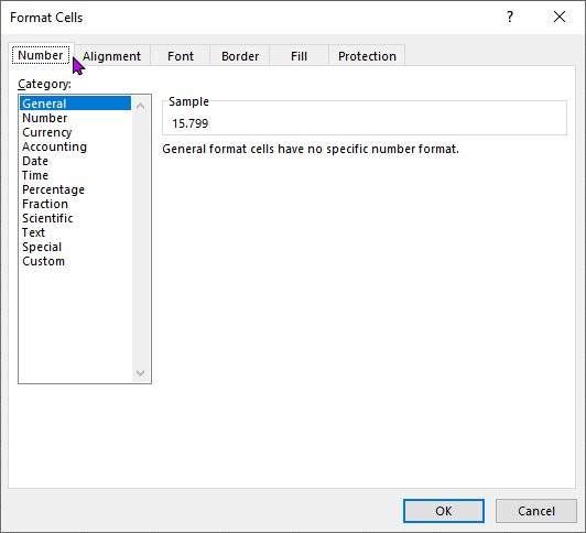
The dialogue window has several tabs (Number, Alignment, Font, …) and any changes made using it will be applied to the cells that were selected when it was opened.
It shows that the default formatting for the selected cells is General. By choosing the next option in the list of Number formatting option such as number of decimal places after the decimal point may be selected. The choice made below is:
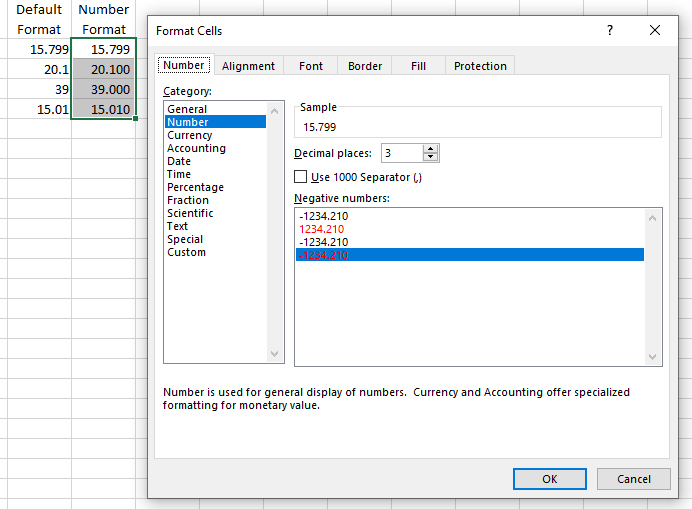
To the left of the dialogue are three cells showing the numbers entered as they are displayed by default (using the General format). To their right they are repeated with the formatting changed to Number. Decimal places has been changed from 2 to 3. The other change made, although not one that affects the currently entered numbers in these cells is that negative numbers will be displayed in red with a minus sign at the beginning of the number.
The same numbers have been repeated in a third column and the Format Cells option used to change the formatting to Currency.
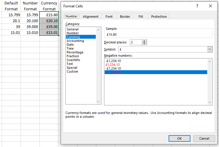
Using the Currency formatting options the decimal places has been changed to 2 decimal places and the symbol option changed to Pounds Sterling. The numbers entered were to three decimal places 9and the the three numbers after the decimal place are still in the cell but only two are being displayed. By default they are rounded up in the conventional manner. How numbers are rounded and the choice of currency symbol may be varied but that is beyond the scope of this article.
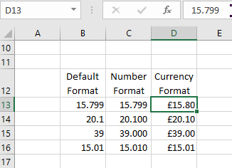
In the above image the cell selected is D13 (the intersection of column D and row 13) and it displays £15.80. at the top of the image it references D13 and then to the right shows the actual content of the cell as 15.799. As the cell is only displaying to two decimal places the numbers has been round up to 15.80 and as the cell is formatted as Currency and to show a Pounds Sterling symbol it appears as £15.80.
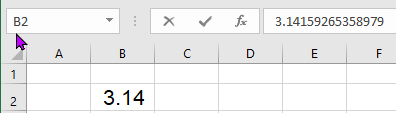
This example demonstrates how deciding of formatting of cells is separate from the actual content of the cell. For example it is possible to enter the value of pi to 14 characters yet display it as a number to just two decimal places as shown below:
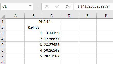
In general most spreadsheets have numbers in them that are used in some form of calculation. Pi may be added to a spreadsheet to calculate the area of a number of circles using the formula
pi times the radius squared (A = π r²)
By entering pi to many decimal places the accuracy of the calculation will be improved but it may not be desired to show pi to the number of decimal places used in the calculation.
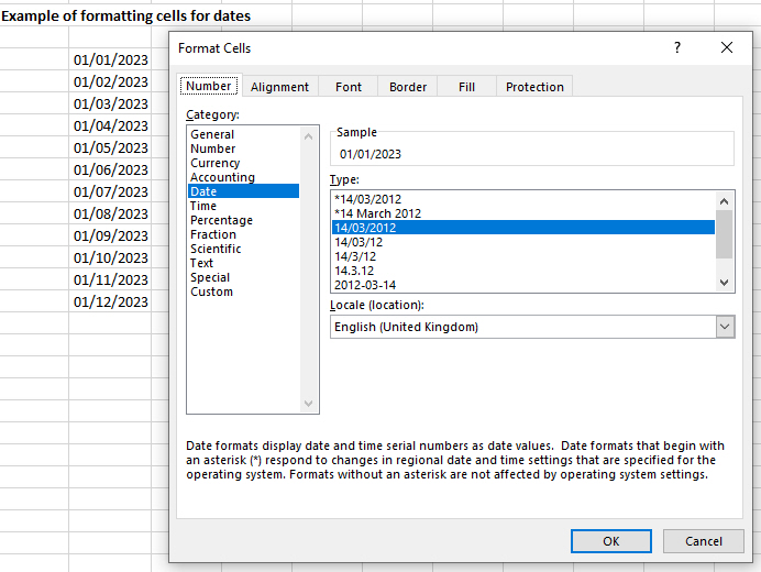
An example of formatting so that Excel understands that a date is being entered into cell and to ensure they are displayed consistently. In this example the first day of each month is displayed and the cells formatted to display the date in the format dd/mm/yyyy as shown:
Using the same twelve cells holding the same data the example shows using a Custom format to display the full name of each month as shown:
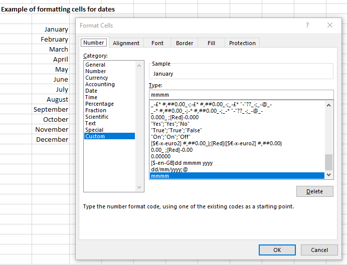
Under the Number tab the Custom category was selected and the Type mmmm entered. These dates now display as January, February etc.
A final example is an interesting extension of this to show the start day of the month for each month of 2023 as shown:
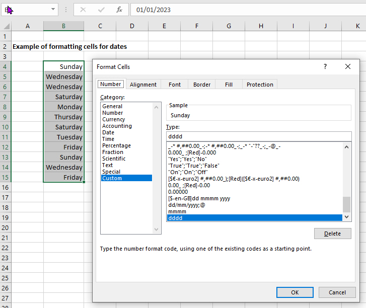
Under the Number tab the Custom category was selected and the Type dddd entered. These dates now display as Sunday (for 1st January 2023), Wednesday (for 1st February 2023) and so on.
A follow-on article will take this further and involve the use of functions to calculate information from other data within a spreadsheet. This may be as simple as adding together numbers held in a group of cells, calculating the number of days between two dates or showing up problems with information in a spreadsheet.