In the article on Formatting in Microsoft Excel it ended up discussing the use of formulas such as adding together numbers held in a group of cells, calculating the number of days between two dates or showing up problems with information in a spreadsheet. This article introduces formulas. Before getting to grips with formulas it is worth understanding formatting of cells as covered in the previous article and how spreadsheets are organised and the elements of the spreadsheet referenced.

Microsoft Excel is just one spreadsheet program but they all (dangerous statement to make) follow the same basic principles.

A spreadsheet is based on a 2 dimensional grid of cells where each cell may be uniquely identified by the X coordinate and the Y coordinate. That sounds complicated but isn’t really. Here is part of a spreadsheet from Excel:

Each cell in the spreadsheet may be identified by the horizonal X coordinate (A, B, C, …) and the vertical Y coordinate (1, 2, 3, …). Rather than say X & Y coordinates the terms used are columns and rows. So a particular cell in the spreadsheet is identified as C3 or G20 as shown below:

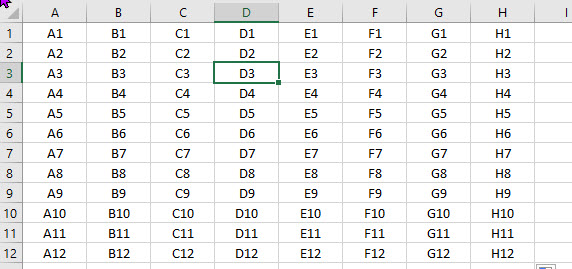
Some points to note are that columns can vary in width and rows vary in height. To work on a particular cell you click the mouse in the relevant cell. Once selected you may make changes to its content. In the above example, the cell D3 is selected and this indicated by the cell’s outline being bolded. Also, it is possible to format the content of a cell and to also format how how a cell is displayed. So, a cell may be given a coloured background and the font have its colour changed. It may be right justified, left justified etc. The content may be formatted so it displays as a date or as currency. Numbers (including currency) may be formatted to have decimal places or not have decimal places. Currency may display a currency symbol such as the £, the $ or the € and many more symbols.

In the following example each cell has the identical value of 100.11 in it but the cells are treating the display of the number differently in each column and the formatting of the cell differently in each row.

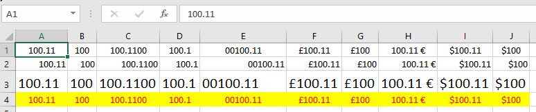
At the top left of the example the spreadsheet is showing the content of the cell A1 as 100.11. Below this we see the cells making up the spreadsheet.

• Row 1 has the contents of the cells centre-justified.
• Row 2 has the contents of the cells right-justified.
• Row 3 has the contents of the cells left-justified. Additionally the text is formatted to be a larger size.
• Row 4 is, again, centre-justified with the text in red and the cell’s background yellow.

• Column A displays the number to two decimal places
• Column B displays the number without decimal places – the cells of this column still contain 100.11 but the .11 is not displayed.
• Column C displays the number to four decimal places – the cells of this column still contain 100.11 but the .1100 is displayed. Column C is also wider than the other columns
• Column D displays the number to one decimal place.
• Column E displays the number with five characters to the left of the decimal place. The number is still 100.11 in each cell of this column. This is unlikely to be used for most numbers but could be useful where numbers are used to represent part numbers in a production or sales operation.
• Column F displays the number to two decimal places as Pounds Sterling currency using the £ symbol. The number is stll 100.11 but it represents currency.
• Column G displays the number without decimal places as Pounds Sterling currency using the £ symbol. The number is still 100.11 but it represents currency.
• Column H displays the number to two decimal places as Euros. The Euro symbol is shown after the currency value.
• Columns I and J are identical in content to columns F & G but the currency is dollars.

A Warning

When using Excel if you enter something into a cell and the width of the cell is too narrow to display it then it will show #######. Just make the column wider and the information entered or the formula’s result will be displayed.

A Simple Formula

In a spreadsheet you enter data and formulas. Data may be numbers, dates and text. Formulas are prefixed with an equal sign (=). An advanced user may well question this division between data and formulas but it generally holds true. If new to spreadsheets you may wish to try this out by creating these examples.

A simple formula might be =1+1 which would show up in the spreadsheet with the answer 2. Not very useful or interesting. More likely, a simple formula (placed in cell A3) might be =A1+A2 in which case the A3 would show an answer based on the contents of A1 and A2. If A1 held the value 999 and A2 held the value -1 the answer shown in A3 would be 998. More interesting and slightly more useful. Addng together more numbers would be soul destroying if we had to reference each cell holding a number. More likely the numbers to be added would be in several cells and it would be better to use a function. Probably the most common function used is Sum. So lets add up the contents of cells A1, A2 through to A10 and place the result in cell A11 as shown below:

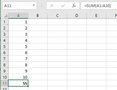
Above the cells the formula used is shown as =SUM(A1:A10). The equals tells Excel to treat it as a formula. SUM is the function and between the parenthesis is the information about what to add up (technically known as the function’s arguments). A1:A10 is a shorthand for saying all cells starting with A1 up to and including A10. What if for some reason the answer should always be one more, then we could change the formula to be =SUM(A1:A10,1). Now we have two arguments in the SUM function which adds the contents of cells A1 to A10 together and then adds the second argument to it, in this case the value one.

Let’s take a further step and add together the contents of the cells A1 to A10 and B1 to B10 as shown below:

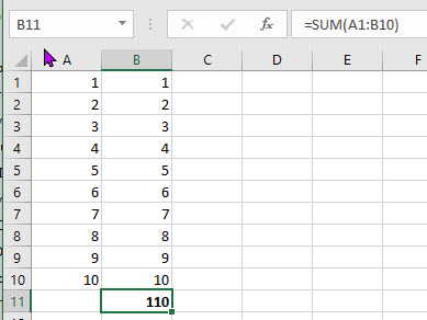
The new formula being used in cell B11 is =SUM(A1:B10). As before the = tells Excel it is a formula and SUM is the function. The argument used with the SUM unction is A1:B10 so Excel is being asked to add together the contents of cells A1 to A10 and B1 to B10. We could have written this formula in a couple of different ways such as =SUM(A1:A10,B1:B10). Just a warning, formulas should not contain spaces. If we wanted to add one to the result the formula may be SUM(A1:A10,B1:B10,1) so it now uses three arguments, the A1:A10, the B1:B10 and the value 1.

Not explained above is that we can change the content of any of teh cells A1 to B10 and the result shown in B11 will be updated automatically. That plus the ability of Excel to copy and paste formulas and for formulas to use the results of other formulas is where the power of a spreadsheet is derived.

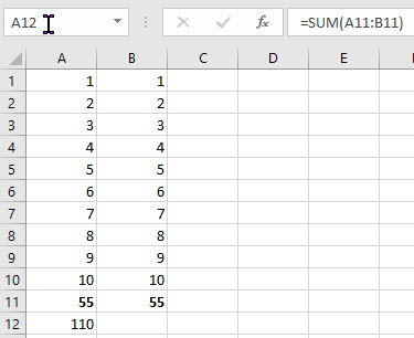
in the above example cell A11 contains the formula =SUM(A1:A10), B11 contains the formula =SUM(B1:B10) and cell A12 contains the formula =SUM(A11:B11). So, cell A11 has the result of adding cells A1 to A10 together, cell B11 has the result of adding cells B1 to B10 together and cell A12 has the result of adding cells A11 and B11 together. This is much closer o how I might create a spreadsheet. In general when i use a function the arguments i will give it are cell references rather than value. That way all the values used by the spreadsheet are visible.

Several Formulas and Functions

The following is much closer to a real-life spreadsheet. The BAHS in the past charged members £3 and visitors £5 to attend lectures. Expenditure tended to be hall hire and the lecturer’s fee. This spreadsheet records the income and expenditure of a lecture and shows the profit or loss.

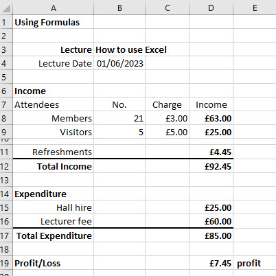
The top of the spreadsheet contains text about the purpose of the spreadsheet including the date of the lecture in cell B4. This cell has been formatted to display dates in style dd/mm/yyyy.

Rows 6 to 12 contain the data and formulas about income. Rows 14 to 17 contain the data and formulas about expenditure. Row 19 shows the profit and loss. Some cells have been formatted to use underlines and bold font. Column widths have been made wider where needed.

Cells B8 and B9 have been formatted to show numbers without decimal places (as it is unlikely a tenth of a person would attend).Cells C8, C9, D8 and D9 have been formatted to show currency with a leading pounds sterling symbol and two decimal places. In Excel parlance we could refer to these four cells as C8:D9. A number of other cells have been formatted to show their content in pounds sterling.

The following example is the same spreadsheet but an excel feature has been used to show the spread as formulas:

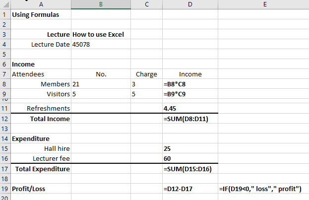
• The lecture date in cell B4 shows up as the value 45078. This is a clue that dates are represented internally within Excel (and computers in general) as numbers.
• Formulas are shown as starting with an = sign. In cell D8 the formula is =B8*C8. This multiplies the number of members by the charge for attending a lecture of 3 (which is formatted as currency). Cell D9 foes a similar thing with visitors.
• In cell D12 the formula =SUM(D8:D11) add together the income from members, visitors and for refreshments taken. It also adds the value in D10 which is empty – row 10 is just used for formatting purposes.
• Cell D17 does a similar job of adding up the expenditure.
• Cell D19 calculates using the formula =D12-D17 whether a profit or loss was made by subtracting expenditure from income.
• The final formula uses a new function which is very useful but takes us into a bit of programming. The value displayed by this formula may be one of two values dependent on the contents of other cells. This iws worth a more detailed study.

The IF Formula

In the example above the cell D19 with the IF function shows the result profit. The example below with the same spreadsheet

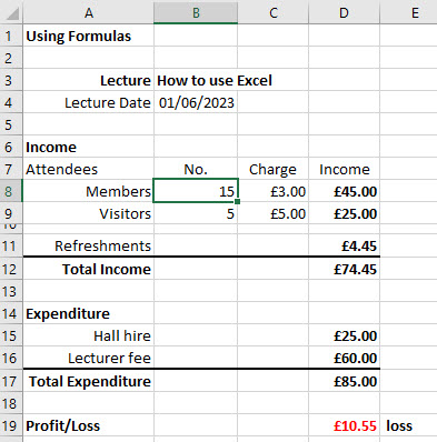
The only difference made is the number of members attending has been changed from 21 to 15. The result is less income and a loss for the event. The cell D19 shows the loss and the formatting of the cell has been set up to show the font in red if it is below zero. Cell E19 shows profit when cell D19 is positive and loss when cell D19 is negative.

The formula used is =IF(D19<0,” loss”,” profit”). The function is IF which is asking a question. The function has three arguments. The first argument is D19<0. The function is asking IF the value in cell D19 less than the value 0. If so it displays the second argument (the IF true argument) which holds the text “profit”. If the value is less that 0 then the third argument (the IF false argument) is displayed which is the text “loss”.

This is a nice demonstration of how text may be represented in a formula by enclosing the text in speech marks. The IF formula could also have used values or cell references for the second and third arguments.

The final point to make about the IF function is that when using the IF function the first argument may evaluate (i.e. result in) a to true of false so it will use a <, >, <=, >=, <> or = between two items being compared whether they are cells or values. Experimentation is key to using this function but it can add a lot to usefulness of a spreadsheet.

Manipulate & Compare Dates

It can be helpful to be able to manipulate and compare dates.

For example you may want to know the date which is 60 days from todays date. To do this format two cells A1 and A2 to show a date in the format of your choice such as dd/mm/yyyy. Then in that cell A1 enter the formula =NOW() If correct this will show today’s date. In cell A2 enter the formula =A1+60.

Another example might be working out how many days you have been on this planet. In cell A1 leave the formula =NOW() and in cell A2 enter your date of birth (in the style you formatted the cell for. if you used dd/mm/yyyy the enter your date of birth in the same style, such as 21-12-2001. Format cell A3 to display a number (no decimal places are required) and enter the formula =A1-A2.

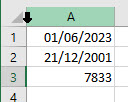
The formula =NOW() in A1 of was entered on the 1st June 2023 so that is why it is showing 01/06/2023.

The formulas used in the above spreadsheet are:

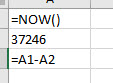
So the answer given is 7833 days. Is it correct? How can you prove the formula works. The biggest risk is that spreadsheets get created, grow in complexity and are not re-validated. Over the years several companies have lost large amounts of money where their estimating spreadsheets for submitting a bid is wrong. Some organisations have and may still use spreadsheets for collecting and analysing significant amounts of data where the risk of incorrect results is high. There is a point where a spreadsheet is not the right answer but a database or a system dedicated to to this type of problem.